Compliant Point Contact

The point contact model defines the contact force by determining the minimum translational displacement (MTD). The minimum translational displacement is the smallest relative displacement between two volumes that will take them from intersecting to just touching. This quantity need not be unique (if two spheres have coincident centers, any direction will serve). Once we have this displacement, we get three quantities that we use to define the contact force:

The direction of the displacement vector is the contact normal.
The magnitude is a measure of the amount of penetration (and is correlated with the magnitude of the normal component of the contact force).
Two witness points for the MTD. The witness points comprise one point on the surface of each volume such that when we apply the minimum translational displacement, they are coincident. We use the witness points (and other physical parameters) to define the point at which the contact force is applied.

This model is simple to implement and cheap to compute, but has some drawbacks.

A single measure of “maximum penetration” cannot distinguish between a large intersecting volume and a small intersecting volume (see Figure 1). The two intersections would produce the same amount of contact force despite the fact that one is clearly compressing more material.
Contact along a large interface is treated as contact at a single point (see Figure 2). Effects that depend on a contact interface over a domain with non-zero area disappear (e.g., torsional friction).
The witness points are not necessarily unique. This means, generally, there is no guarantee that the witness points will be consistent from frame to frame, which means that the point at which the force is applied will not be consistent. This can produce non-physical artifacts like sudden changes in force direction.

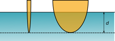
Figure 1: Two intersections with significantly different intersecting volumes characterized with the same measure: d.

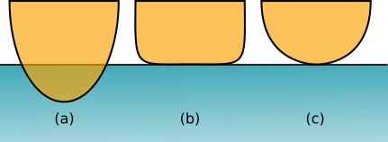
Figure 2: Modeling contact forces with point contact (considering the blue half space as rigid). (a) the actual intersection of the simulated bodies. (b) the conceptual deformation of the orange body creating a large area of contact. (c) how point contact sees the deformation: contact at a single point.

Modeling of Forces

Given the "maximum penetration" x, we compute the normal component of the contact force according to a simple compliant law of the form:

   fₙ = k(x)₊(1 + dẋ)₊

with (a)₊ = max(0, a). The normal contact force fₙ is made a continuous function of the penetration distance x between the bodies (defined to be positive when the bodies are in contact) and the penetration distance rate ẋ (with ẋ > 0 meaning the penetration distance is increasing and therefore the interpenetration between the bodies is also increasing). Stiffness k and dissipation d are the combined "effective" stiffness and dissipation for the pair of contacting geometries. Dissipation is modeled using a Hunt & Crossley model of dissipation, see Modeling Dissipation for details. For flexibility of parameterization, stiffness and dissipation are set on a per-geometry basis (Accessing point contact parameters). Given two geometries with individual stiffness and dissipation parameters (k₁, d₁) and (k₂, d₂), we define the rule for combined stiffness (k) and dissipation (d) as:

  k = (k₁⋅k₂)/(k₁+k₂)
  d = (k₂/(k₁+k₂))⋅d₁ + (k₁/(k₁+k₂))⋅d₂

These parameters are optional for each geometry. For any geometry not assigned these parameters by a user Pre-Finalize, MultibodyPlant will assign default values such that the combined parameters of two geometries with default values match those estimated using the user-supplied "penetration allowance", see Default Parameters.

Note: When modeling stiff materials such as steel or ceramics, these model parameters often need to be tuned as a trade-off between numerical stiffness and physical accuracy. Stiffer materials lead to a harder to solve system of equations, affecting the overall performance of the simulation. The convex approximations provided in Drake are very robust even at high stiffness values, please refer to [Castro et al., 2023] for a study on the effect of stiffness on solver performance.

Default Parameters

Note: The treatment of default parameters is undergoing a major revision. Please refer to the documentation for DefaultProximityProperties and for AddMultibodyPlant(). For now, we still support the "penetration allowance" workflow outlined below, but that might change.

While we strongly recommend setting these parameters appropriately for your model, MultibodyPlant aids the estimation of these coefficients using a heuristic function based on a user-supplied "penetration allowance", see set_penetration_allowance(). This heuristics offers a good starting point when creating a simulation for the first time. Users can then set material properties for specific geometries once they observe the results of a first simulation with these defaults. The penetration allowance is a number in meters that specifies the order of magnitude of the average penetration between bodies in the system that the user is willing to accept as reasonable for the problem being solved. For instance, in the robotic manipulation of ordinary daily objects the user might set this number to 1 millimeter. However, the user might want to increase it for the simulation of heavy walking robots for which an allowance of 1 millimeter would result in a very stiff system.

As for the dissipation coefficient in the simple law above, MultibodyPlant chooses the dissipation coefficient d to model inelastic collisions and therefore sets it so that the penetration distance x behaves as a critically damped oscillator. That is, at the limit of ideal rigid contact (very high stiffness k or equivalently the penetration allowance goes to zero), this method behaves as a unilateral constraint on the penetration distance, which models a perfect inelastic collision. For most applications, such as manipulation and walking, this is the desired behavior.

When set_penetration_allowance() is called, MultibodyPlant will estimate reasonable stiffness and dissipation coefficients as a function of the input penetration allowance. Users will want to run their simulation a number of times to determine if they are satisfied with the level of inter-penetration actually observed in the simulation; if the observed penetration is too large, the user will want to set a smaller penetration allowance. If the system is too stiff and the time integration requires very small time steps while at the same time the user can afford larger inter-penetrations, the user will want to increase the penetration allowance. Typically, the observed penetration will be proportional to the penetration allowance. Thus scaling the penetration allowance by say a factor of 0.5, would typically results in inter-penetrations being reduced by the same factor of 0.5. In summary, users should choose the largest penetration allowance that results in inter-penetration levels that are acceptable for the particular application (even when in theory this penetration should be zero for perfectly rigid bodies.)

For a given penetration allowance, the contact interaction that takes two bodies with a non-zero approaching velocity to zero approaching velocity, takes place in a finite amount of time (for ideal rigid contact this time is zero.) A good estimate of this time period is given by a call to get_contact_penalty_method_time_scale(). Users might want to query this value to either set the maximum time step in error-controlled time integration or to set the time step for fixed time step integration. As a guidance, typical fixed time step integrators will become unstable for time steps larger than about a tenth of this time scale.

Choosing the Right Collision Geometry

The compliant point contact model only reports a single contact between bodies. More particularly, the contact is characterized by a single point. In some cases (e.g., a steel ball on a table surface), that is perfectly fine. For objects that contact across a large surface area (such as a box on the table), this characterization has two negative implications:

the contact point will not be guaranteed to be at the center of pressure, possibly inducing unrealistic torque, and
not be temporally coherent. This will lead to instability artifacts which can only be addressed through smaller time steps.

Both of these issues can be addressed by changing the geometry that represent the body's contact surface. For some shapes (e.g., boxes), we can introduce two sets of collision elements: discrete "points" at the corners, and a box capturing the volume (see block_for_pick_and_place.urdf and inclined_plane_with_body.cc in Drake's examples). With this strategy, the contact "points" are actually small-radius spheres. The volume-capturing box should actually be inset from those spheres such that when the box is lying on a plane (such that the logical contact manifold would be a face), only the contact points make contact, providing reliable points of contact. However, for arbitrary configurations contact with the box will provide more general contact.

The Hydroelastic contact model described below in Hydroelastic Contact, was designed to resolve these issues in a principled manner. We recommend switching to this model unless other requirements such as simulation speed are a constraint.

Hydroelastic Contact

The purpose of this documentation is to provide a quick overview of the Hydroelastic contact model and its modeling parameters. More details are provided in Drake's Hydroelastic Contact User Guide and references therein.

Hydroelastic contact was created to address some of the short-comings in point contact. In fact, one might argue that many of the strategies used to mitigate the shortcomings of point contact (such as using lots of points) push it closer and closer to hydroelastic contact.

Hydroelastic Contact was originally introduced by [Elandt et al., 2019]. Modifications and further development of the model can be found in [Masterjohn et al., 2022]. In Drake, we refer to this model as the “hydroelastic” model. It differs from point contact in how it characterizes the contact. Rather than a single point, it imagines an entire contact surface. This surface is an approximation of the contact surface as visualized in Figure 2(b).

When two objects come into contact, forces are produced due to deformation ("strain") of the objects at the contact interface. At first touch, there are no forces but as the objects are pressed further they deform to produce a region over which contact pressure is non-zero, causing equal-and-opposite forces to act on the objects. Calculating the actual deformations is expensive. Hydroelastic contact is based on the idea that for relatively small deformations we can approximate the resulting contact interface and pressure distribution without having to compute the actual deformations. We do that by precalculating a "pressure field" on the interior of compliant objects (see Figure 3). The pressure field approximates the pressure that would result from deforming the surface to some point within the field. A point on the surface (that is, no deformation) experiences zero pressure, but as it is pressed inward, it experiences an increase in pressure (up to a maximum pressure on the interior of the body). When two bodies are colliding, we look for a surface in the intersecting volume where the pressure on the surface is the same in each object; it’s an equilibrium surface (see Figure 4). There is pressure defined across the entire contact surface. It is integrated to define the resultant contact force and moment.

Figure 3: Three shapes and possible pressure fields in the interior of the object. Pressure is zero at the outer boundary, and maximum on the interior.

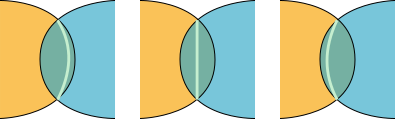
Figure 4: The equilibrium contact surface (pale green) between two bodies where the left-hand, yellow body has (a) less compliance, (b) equal compliance, and (c) greater compliance.

This equilibrium surface has important properties:

The contact surface will always be contained within the intersecting volume.
The surface’s edge will always lie on the surface of both objects and have zero pressure.
The location of the surface depends on the relative compliance of the two objects. As one object becomes more rigid than the other, the contact surface begins to converge to its surface (see Figure 4). As one surface becomes perfectly rigid, the other object deforms completely to conform to its shape.
The contacting bodies need not be convex, nor will the contact surface between two objects necessarily be a single contiguous patch. For non-convex geometries, the contact can be meaningfully represented by multiple disjoint patches. The resultant contact force will still be meaningful.
The resultant contact force is continuous with respect to the relative pose between bodies. In fact, the contact surface’s mesh, its area, and the pressures measured on the surface are likewise continuous.

Model Parameters

The hydroelastic modulus has units of pressure, i.e. Pa (N/m²). The hydroelastic modulus is often estimated based on the Young's modulus of the material though in the hydroelastic model it represents an effective elastic property. For instance, [Elandt et al., 2019] chooses to use E = G, with G the P-wave elastic modulus G = (1-ν)/(1+ν)/(1-2ν)E, with ν the Poisson ratio, consistent with the theory of layered solids in which plane sections remain planar after compression. Another possibility is to specify E = E*, with E* the effective elastic modulus given by the Hertz theory of contact, E* = E/(1-ν²). In all of these cases a sound estimation of hydroelastic_modulus starts with the Young's modulus of the material. However, due to numerical conditioning, much smaller values are used in practice for hard materials such as steel. While Young's modulus of steel is about 200 GPa (2×10¹¹ Pa), hydroelastic modulus values of about 10⁵−10⁷ Pa lead to good approximations of rigid contact, with no practical reason to use higher values.

Note: Although the hydroelastic modulus carries the same units as the more familiar elastic moduli mentioned above, it is qualitatively different. Do not expect to use values for those moduli for the hydroelastic modulus to good effect.

As with point contact, the hydroelastic contact model uses a Hunt & Crossley dissipation model (see Modeling Dissipation). It differs in defining the combined effective dissipation parameter; for hydroelastic contact, the combined dissipation depends on the hydroelastic moduli of the contacting geometries. For two hydroelastic bodies A and B, with hydroelastic moduli Eᵃ and Eᵇ, respectively, and dissipation dᵃ and dᵇ, respectively, the effective dissipation is defined according to the combination law:

  E = Eᵃ⋅Eᵇ/(Eᵃ + Eᵇ),
  d = E/Eᵃ⋅dᵃ + E/Eᵇ⋅dᵇ = Eᵇ/(Eᵃ+Eᵇ)⋅dᵃ + Eᵃ/(Eᵃ+Eᵇ)⋅dᵇ

thus dissipation is weighted in accordance with the fact that the softer material will deform more and faster and thus the softer material dissipation is given more importance.

The hydroelastic user guide shows how values for these properties can be assigned to geometries.

Hydroelastic Contact in practice

The theory operates on arbitrary geometries and pressure fields. In practice, we operate on discrete representations of both the geometry and the field.

Compliant objects are represented by tetrahedral meshes. The Drake data type is VolumeMesh. The pressure fields on those meshes are piecewise linear.

The resulting contact surface is likewise a discrete mesh. This mesh may be built of nothing but triangles or polygons. The choice of representation has various implications on the computation of contact forces (see below). The pressure on the contact surface is likewise a piecewise linear function.

Objects with very large hydroelastic modulus can introduce stiffness into the numerics of the contact resolution computation and lead to ill conditioning, affecting simulation performance and robustness. For these cases, Drake permits declaring an object as "rigid hydroelastic" (see Creating hydroelastic representations of collision geometries.) When a rigid hydroelastic object interacts with other compliant hydroelastic objects, the contact surface always follows the surface of the rigid object. Think of it as the compliant object doing 100% of the deformation, so it conforms to the shape of the rigid object. However, rigid hydroelastic objects have limitations. There is no hydroelastic contact surface between two rigid hydroelastic representations – when contact is observed between two such objects, the contact will be characterized with point contact (or maybe even throw), depending on how the contact model has been configured. For this reason, the use of the rigid hydroelastic declaration should be used judiciously – making everything compliant can be simpler in reasoning about the scene.

Important points to note:

The time cost of resolving contact scales with the complexity of the contact surface (number of faces).
The complexity of the contact surface is a function of the complexity of the contacting geometries.
The best performance comes from the lowest resolution meshes that produce “acceptable” behaviors.
It is not universally true that every geometry is represented discretely. The implementation may represent some shapes differently when it allows performance improvements. The canonical example would be a half space geometry. As a shape with infinite volume, it would be infeasible to create a finite, discrete representation. It is also unnecessary. Intersecting meshes directly with a half space is far more efficient.

Modeling Dissipation

We use a dissipation model inspired by the model in [Hunt and Crossley 1975], parameterized by a dissipation constant with units of inverse of velocity, i.e. s/m.

To be more precise, compliant point contact forces are modeled as a function of state x:

  f(x) = fₑ(x)⋅(1 - d⋅vₙ(x))₊

where here fₑ(x) denotes the elastic forces, vₙ(x) is the contact velocity in the normal direction (negative when objects approach) and (a)₊ denotes "the positive part of a". The model parameter d is the Hunt & Crossley dissipation constant, in s/m. The Hunt & Crossley term (1 - d⋅vₙ(x))₊ models the effect of dissipation due to deformation.

Similarly, Drake's hydroelastic contact model incorporates dissipation at the stress level, rather than forces. That is, pressure p(x) at a specific point on the contact surface replaces the force f(x) in the point contact model:

  p(x) = pₑ(x)⋅(1 - d⋅vₙ(x))₊

where pₑ(x) is the (elastic) hydroelastic pressure and once more the term (1


d⋅vₙ(x))₊ models Hunt & Crossley dissipation.

This is our preferred model of dissipation for several reasons:


It is based on physics and has been developed based on experimental observations.
It is a continuous function of state, as in the real physical world. Moreover, this continuity leads to better conditioned systems of equations.
The bounce velocity after an impact is bounded by 1/d, giving a quick physical intuition when setting this parameter.
Typical values are in the range [0; 100] s/m, with a value of 20 s/m being typical.
Values larger than 500 s/m are unphysical and usually lead to numerical problems when using discrete approximations given how time is discretized.

The Hunt & Crossley model is supported by the drake::multibody::DiscreteContactApproximation::kTamsi, drake::multibody::DiscreteContactApproximation::kSimilar, and drake::multibody::DiscreteContactApproximation::kLagged model approximations. In particular, drake::multibody::DiscreteContactApproximation::kSimilar and drake::multibody::DiscreteContactApproximation::kLagged are convex approximations of contact, using a solver with theoretical and practical convergence guarantees.